Tidal Visualization with Didactic Pattern Visualizer

Developer	Iván Abreu
Source code	GitHub
Visualizing Application	Processing
Blog post	HighHarmonics

Introduction

Didactic Pattern Visualizer (DPV) is an easy way to visualize sound patterns from Tidal Cycles. It was created by the artist and creative technologist Iván Abreu "...to study the potential and complexity of the syntax of the pattern system for sequencing Tidal Cycles sounds." It utilizes the open source visualization program Processing to provide a scrolling grid where colored shapes appear in rhythm reflecting the flow of Tidal events (notes). The GitHub materials also includes Tidal Cycles examples using DPV by the musician and digital Artist CNDSD.

To use DPV (summary):

• Install and configure the Processing application to receive OSC messages from Tidal
• Load the OSC and Tidal configurations each time you use it (or load it with your BootTidal.hs)
• Set the scrolling grid parameters for your Tidal session
• Add a connection parameter to each pattern you want to visualize

Installation

The GitHub source includes a detailed installation/configuration guide. The main step is to install the Processing application and add the oscP5 library file. You also need to download the Processing runtime pde files that make up the DPV codebase.

OSC targets

DPV leverages the ability of Tidal to send OSC messages to multiple targets (which is covered in the Tidal OSC docs.) DPV listens to OSC messages on port 1818. With the dual targets, every Tidal channel that has the "connectionN" parameter set will display the visual representation of notes.

Examples

The Readme page includes an good set of examples that include Tidal code along with mp4 files that play the audio with visualizations. There is also musical examples and code provided by the digital artist CNDSD - well know for expanding boundaries in live coding and interdisciplinary art forms.

Usage

In the ReadMe, Iván notes that there are multiple ways to use DPV:

• As a tool for composing - for the visual feedback of ordering and sound intentions.
• During live performance, to help unfold the musical structure and then emphasize and direct attention to rhythmic interactions of multiple sound layers.

Creative Example - composed live code with visualization

The example below shows how I used DPV to support composing prepared code with rhythmic patterns that use cross-rhythms, polymeter, and irregular beat patterns. I found it to be really helpful to see exactly what is happening within the cycles and observing how the note placements change as I make small adjustments to pattern values.

• Screen recording of the full session: Erratic Rhythms with visualization
• Tidal code: GitHub - Erratic Rhythms

Description

Erratic Rhythms has 4 separate parts, each with its own distinct rhythmic character. The patterns were created so that each part stands out without "lining up" on the beats. The piece evolves so that the parts are played in different groups of 2 and 3 parts sounding together. Each part has a different timbre, using synthesizers available in SuperDirt (superhex, psin, supergong, soskick).

The organizing idea is to have fully independent parts - each with a distinctive character - that still work well together. To ensure part independence, I keep the rhythmic values of each part sounding in different parts of the beat. That is where the visualization and DPV really helped. During the stage of code preparation, I would experiment with different pattern values and closely watch the visualizations to see where the rhythms land, and then make adjustments to find the right values. During a performance session, I improvise on the prepared code options and use the visualization to give me a sense of how everything fits together and what I should do next.

Examples - Erratic Rhythms

1 play

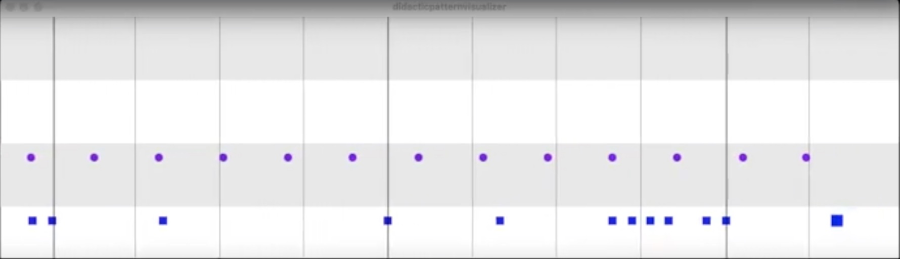
• d1 (lower part): 8 beat pattern on the beat with regular subdivisions
• d2 (upper part): 9 note pattern using a polymetric subdivision value of %5.2 and nudge 0.2

d1 $ freq "[70 ~ 800] [<500 ~ > < ~ ~ <300*2 300*3> > [1170 ~ 900]]" # sound "superhex"
  # connectionN 4 # sizeMin 12 # sizeMax 80 # figure "rect" # color "0519f5" -- DVP OSC values

d2 $ freq "{100 200 400 800 900 1100 1300 1500 1600}%<5.2>" # sound "psin"  #nudge 0.2
  # connectionN 3 # sizeMin 12 # sizeMax 60 # color "8905f5"

2 play

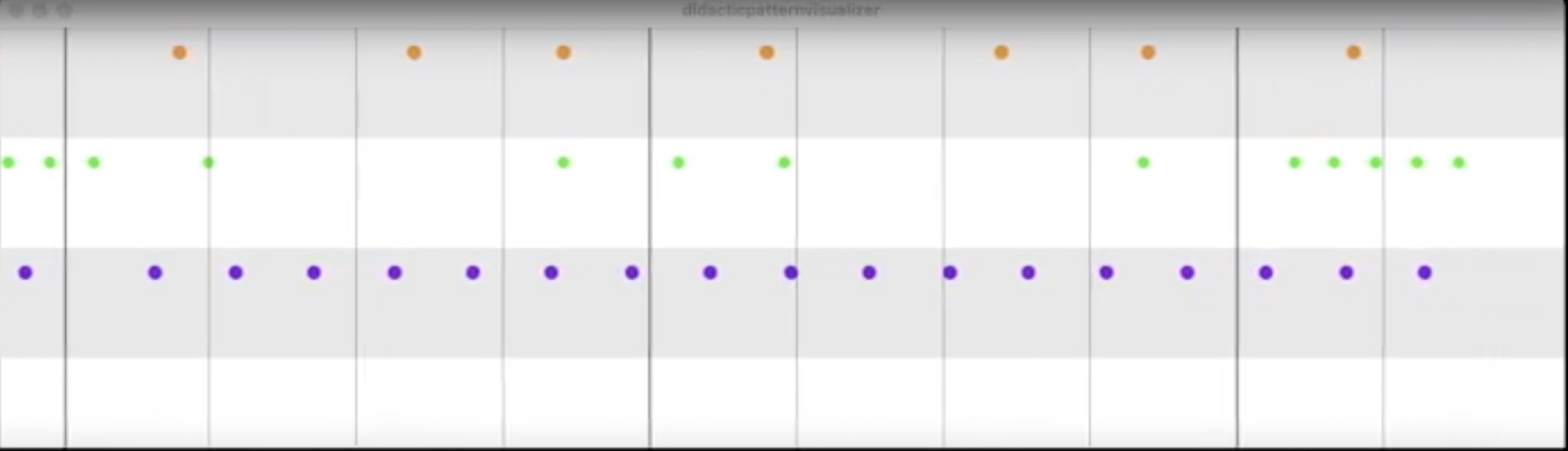
• d2 (lower): 9 note pattern, with polymetric subdivision value of %7.4
• d3 (middle): )17 note pattern with different metric divisor values [supergong!17]/<3.4 5.2 1.2> pattern speed changes with each cycle
• d4 (upper): 3 notes against 5 beats with notes offset with rests

d2 $ freq "{100 200 400 800 900 1100 1300 1500 1600}%<7.4>" # sound "psin"

d3 $ mask ("1 0 1") $ s "[supergong!17]/<3.4 5.2 1.2>" #nudge 0.2
  # connectionN 2 # sizeMin 10 # sizeMax 20 # figure "circle" # color "2df505"

d4 $ freq "~ 400 ~ 800 [~ <1300 1600> ~ ~]" # s "soskick"
  # connectionN 1 # sizeMin 12 # sizeMax 80 # figure "circle" # color "f58711"

3 play

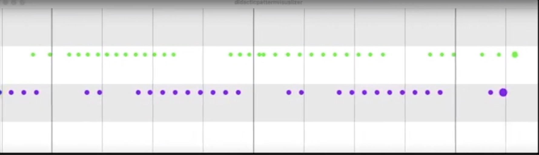
• d2: 9 note pattern with polymetric subdivision of 16
• d3: 17 note pattern with alternating polymetric subdivisions %<1 1.4 0.8>

d2 $ freq "{1100 200 400 800 900 1100 1300 1500 1600}%16"  # sound "psin"

d3 $ mask ("1 1 1 0 1") $ sound "[supergong!17]/<1 1.4 0.8>" #nudge 0.2
   #connectionN 2 #sizeMin 10 #sizeMax 20 #figure "circle" #color "2df505"

4 play

d2 $ jux (rev) $ freq "{100 200 400 800 900 100 1300 1500 1600 1800 2100 2400 ~}%11"  # sound "psin"
  # connectionN 3 # sizeMin 12 # sizeMax 60 # color "8905f5" # nudge 0.2

d3 $ jux (rev) $ sound "[supergong!17]/<0.6 1>" # nudge 0.3
  # connectionN 2 # sizeMin 10 # sizeMax 20 # figure "circle" # color "2df505"

d4 $ fast 0.5 $ every 2 (degradeBy "<0.2 0.5 0.8>") $ freq ("~ 400 ~ 800 [~ <1300 1600> ~!2]" |* 0.5) # s "soskick"
    # connectionN 1 # sizeMin 12 # sizeMax 80 # figure "circle" # color "f58711"

So that's it!

• Full performance: Erratic Rhythms - with visualization
• Tidal code: GitHub - Erratic Rhythms

Check out Iván's Didactic Pattern Visualizer

HighHarmonics